| METHOD: | Grand-canonical transition-matrix Monte Carlo [1] |
| V/σ3: | 512 |
| TRUNCATION: | 3σ + standard long range corrections |
| Prob. of Disp. Move: | 0.75 |
| Prob. of Ins/Del. Move: | 0.25 |
| Biasing Function Update Frequency: | 1.0E6 trials |
| Simulation Length: | 8.0E9 trials |
| Choose a temperature to jump to table of pressure versus density data | |||||||||||||||||
| kBT/ε = | 0.70 | 0.75 | 0.80 | 0.85 | 0.90 | 0.95 | 1.00 | 1.05 | 1.10 | 1.15 | 1.20 | 1.25 | 1.30 | 1.35 | 1.40 | 1.45 | 1.50 |
RAW Simulation Data:
For each temperature, five raw macrostate (particle number) distributions are provided (gzipped tar files). Also included is the average total potential energy (dimensionless) of a given macrostate. The first column in each file represents N, the number of particles, and the second column represents ln Π (N), the natural logarithm of the probability of observing N particles given the conditions of the simulation (fixed chemical potential, volume, and temperature). The information required to manipulate the macrostate distributions are listed below.
| kBT/ε | Nmin | Nmax | ln zsim |
|---|---|---|---|
| 0.70 | 0 | 475 | -5.943376 |
| 0.75 | 0 | 475 | -5.400601 |
| 0.80 | 0 | 470 | -4.937419 |
| 0.85 | 0 | 470 | -4.540504 |
| 0.90 | 0 | 465 | -4.200008 |
| 0.95 | 0 | 465 | -3.867387 |
| 1.00 | 0 | 425 | -3.823078 |
| 1.05 | 0 | 415 | -3.436560 |
| 1.10 | 0 | 400 | -3.245568 |
| 1.15 | 0 | 400 | -3.068218 |
| 1.20 | 0 | 390 | -2.902929 |
| 1.35 | 0 | 380 | -0.9114399 |
| 1.40 | 0 | 375 | -0.7669414 |
| 1.45 | 0 | 370 | -1.940905 |
| 1.50 | 0 | 370 | -1.568214 |
z is the so-called activity which is defined as
z = Λ-3 exp ( βμ )
where Λ is the de Broglie wavelength, β is 1/kBT (kB
is Boltzmann's constant), and μ is the chemical potential.
Remarks:
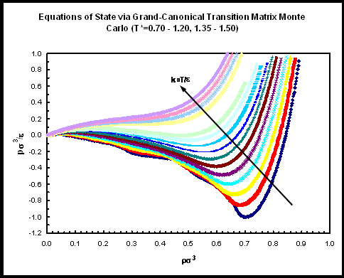
Uncertainties were obtained from 5 independent simulations and represent 67% confidence limits (one standard deviation). Here, an equation of state (pressure as a function of density, at a given temperature) is constructed from the particle number probability distribution (determined by grand-canonical transition-matrix Monte Carlo) by exploiting the fact that the Helmholtz free energy is related to the grand potential by a Legendre transform with respect to particle number. The details of this construction can be found it Ref. 2. It should be pointed out that the apparent van der Waals loops in the isotherms are system-size dependent [2]. Therefore, only the points outside the liquid-vapor coexistence region are expected to be reproduced reliably using system sizes other than that used here.
[1] J. R. Errington, J. Chem. Phys. 118, 9915 (2003).
[2] V. K. Shen and J. R. Errington, J. Phys. Chem B 108, 19595 (2004).
[3] V. K. Shen and D. W. Siderius, J. Chem. Phys., 140, 244106, (2014).
[4] V. K. Shen and J. R. Errington, J. Chem. Phys. 122, 064508, (2005).
[5] V. K. Shen, R. D. Mountain, and J. R. Errington, J. Phys. Chem. B 111, 6198, (2007).
[6] D. W. Siderius and V. K. Shen, J. Phys. Chem. 117, 5681, (2013).