Lennard-Jones fluid simulation website
6. Surface Tension
The interfacial tension between bulk liquid and vapor phases, that is the
surface tension, was determined using two different methodologies, molecular dynamics simulation of the liquid-vapor interface and the
combination of finite-size scaling and grand-canonical Monte Carlo.
[1] Interfacial properties, unlike bulk fluid properties, are sensitive to the
details of the actual potential used in the simulation due to the
inhomogeneous nature of the interface. It is therefore crucial that long range
corrections be treated correctly.
6a. Explicit interfacial simulations:
Molecular dynamics simulations of the liquid-vapor interface
were performed in a
simulation cell of dimensions L
x � L
y � L
z
(where L
x = L
y < L
z).
Long range corrections to the force, energy, and pressure tensor were applied
at every time step using the density-profile-based scheme introduced by
Janecek.
[2] Those who are interested are referred to the Ref.
[2] for the
mathematical expressions and their derivations. The surface tension
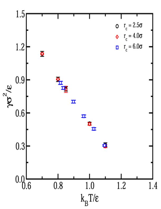
g was calculated by taking the difference in the
diagonal components of the pressure tensor
g = [ 2Pzz
- ( Pxx + Pyy) ] / (2A)
where Pkk is the pressure tensor component and A is the total
interfacial area (A=2LxLy). The surface tension
was determined over the reduced temperature range of 0.70 to 1.10 using cutoff
distances of rc/σ = 2.5, 4.0,
and 6.0. Uncertainties represent the standard deviation of at least three
separate simulations. In all cases, the properties of the coexisting fluid
phases were in excellent agreement with those reported in other pages on this
website. Important details of the simulations are given in the table below:
| ENSEMBLE:: |
Micocanonical (NVE) |
| INTEGRATOR: |
Velocity-Verlet |
| EQUILIBRATION: |
Long enough to stabilize interface |
| PRODUCTION: |
1000 t* |
| TIME STEP: |
0.01 t*
|
| N: |
1600 |
| ( Lx, Ly, Lz
) |
( 12.1σ,
12.1σ, 40σ
) |
| Δz |
0.1σ |
Several simulations with N=2500 and box dimensions 11
σ
� 11
σ � 66
σ
were performed to investigate system size effects. Within the uncertainties,
none were found. An initial configuration was generated by placing a liquid slab
in the middle of an empty tetragaonal simulation box. As long as the overall
density of the system is between that of the saturated vapor and liquid, then
two liquid-vapor interfaces will form. Of crucial importance in an interfacial
simulation is the formation and stabilization of the interface itself. For this
reason, a predetermined equilibration period throughout all the runs was not used.
Rather, the stability of the interface was explicitly checked for each run. In the table below, the mean surface tension and standard
deviation from at least three molecular dynamics simulations are reported. In
all cases, the densities of the coexisting phases were in agreement with
saturation data provided
elsewhere on this website.
| T* |
rc/σ |
γ* |
+/- |
 |
| 0.700 |
2.5 |
1.1356 |
0.022 |
| 0.700 |
4.0 |
1.1367 |
0.006 |
| 0.800 |
2.5 |
0.9043 |
0.002 |
| 0.800 |
4.0 |
0.9057 |
0.003 |
| 0.816 |
6.0 |
0.8720 |
0.014 |
| 0.835 |
6.0 |
0.8260 |
0.013 |
| 0.850 |
2.5 |
0.8175 |
0.019 |
| 0.850 |
4.0 |
0.8130 |
0.028 |
| 0.898 |
6.0 |
0.7026 |
0.013 |
| 0.963 |
6.0 |
0.5743 |
0.011 |
| 1.000 |
2.5 |
0.5037 |
0.012 |
| 1.000 |
4.0 |
0.4993 |
0.012 |
| 1.030 |
6.0 |
0.4554 |
0.011 |
| 1.100 |
2.5 |
0.3107 |
0.018 |
| 1.100 |
4.0 |
0.2973 |
0.013 |
| 1.100 |
6.0 |
0.3050 |
0.006 |
6b. Finite-Size Scaling and
Transition-Matrix Monte Carlo
An alternative route to interfacial tension is the combination of finite-size
scaling and transition-matrix Monte Carlo. [1] This methodology uses grand-canonical
transition-matrix Monte Carlo (GC-TMMC) [6-10] to calculate apparent surface tensions at
various system sizes and then employs finite-size scaling arguments to
extrapolate the data to the thermodynamic limit. As noted on a
previous page, GC-TMMC provides the particle number
probability distribution, that is the the probability of observing N particles
in a simulation box of volume V at temperature T and chemical potential
�. The distribution of interest here is
the one at which the chemical potential corresponds to liquid-vapor phase
coexistence �sat. From this
distribution, an apparent surface tension L can be calculated
where FL is the height of the free energy barrier separating the
two coexisting phases. Since cubic simulation boxes were used here, V = L3.
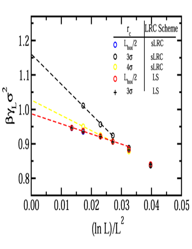
Because FL is system-size-dependent, so too is the apparent surface
tension. The thermodynamic surface tension is obtained by applying the
following scaling proposed by Binder [3]

where c1 and c2 are unknown constants,
β is 1/(kBT), and
γ∞ is the thermodynamic surface
tension. For large L, the apparent surface tension is a linear function of the
scaling variable (ln L)/L2, where the y-intercept corresponds to
the thermodynamic surface tension. For the Lennard-Jones fluid, the linear
scaling regime appears (empirically) to be applicable to for L
≥ 9σ.
The surface tension of the Lennard-Jones fluid was calculated using the
finite-size scaling and grand-canonical transition-matrix Monte Carlo (FSS/GC-TMMC)
methodology. Run parameters are summarized in the table below:
| METHOD: |
GC-TMMC |
| kBT/ε |
0.70, 0.85, and 1.10 |
| Prob. of Disp. Move: |
0.70 |
| Prob, of Ins/Del. Move: |
0.30 |
Biasing Function Update Frequency
|
1 million trials
|
| Simulation Length: |
1 - 20 billion MC trials |
Effect of Truncation Using Standard Long Range Corrections:
At a reduced temperature of 0.85, standard long range corrections (sLRC's)
were used, and three cutoff distances were compared, rc = 3σ,
4σ, and L/2. Phase coexistence properties
obtained for each cutoff were in agreement with data presented
elsewhere. Apparent and thermodynamic (bold) surface tension
data are given below, along with uncertainties which represent the standard
deviation from at least 3 separate simulations per point.
|
rc |
L/σ |
γL* |
+/- |
| 3.0σ |
7 |
0.712 |
0.0003 |
| 3.0σ |
8 |
0.755 |
0.0005 |
| 3.0σ |
9 |
0.785 |
0.0009 |
| 3.0σ |
10 |
0.812 |
0.0004 |
| 3.0σ |
12 |
0.859 |
0.0007 |
| 3.0σ |
∞ |
0.986 |
0.0081 |
| 4.0σ |
8 |
0.747 |
0.0001 |
| 4.0σ |
9 |
0.771 |
0.0006 |
| 4.0σ |
10 |
0.786 |
0.0009 |
| 4.0σ |
12 |
0.808 |
0.0008 |
| 4.0σ |
∞ |
0.873 |
0.0072 |
| L/2 |
7 |
0.712 |
0.0025 |
| L/2 |
8 |
0.750 |
0.0009 |
| L/2 |
9 |
0.771 |
0.0008 |
| L/2 |
10 |
0.783 |
0.0016 |
| L/2 |
12 |
0.795 |
0.0023 |
| L/2 |
14 |
0.804 |
0.0013 |
| L/2 |
∞ |
0.837 |
0.0020 |
An alternative treatment of long-range correction is the lattice summation.
[4,5]
While this is a more robust treatment, it is computationally expensive. The
dominant contribution to the Lennard-Jones pair potential at large separations is the
dispersive (inverse sixth power) term , and therefore, one focuses on the long
range corrections to this contribution. Applying the lattice summation to the dispersive
term of the potential, the total dispersion interaction in a system U6 can be written as
the sum a real-space term and reciprocal space term
 .
.
The real-space contribution to the total dispersion energy is

where Bjk = -BjBk and

In the above expressions, ri is the position of particle i,
RL is a lattice translation vector, and
ν is an adjustable parameter controlling
the range of the real-space interaction. In the literature,
ν is commonly expressed as α/L where α is a
dimensionless parameter and L is the length of the simulation box. The prime in
the summation indicates that terms for which j=k when L=0 are excluded. While
the summation is formally an infinite sum, when evaluated in practice, it is
truncated at L=0 and only to those pairs of particles separated by a distance less
than a cutoff rc.
The reciprocal space contribution to the dispersion interaction is
where S(h) is the structure factor
and the function J(h) is
where h = (2π/L)(kx,ky,kz)
is a reciprocal lattice vector of magnitude h, and V is the system
volume. The summation over h is truncated at some maximum lattice vector
hmax. In practice evaluation of the lattice summation requires
specification of three parameters, rc,
ν, and hmax = (2π/L)kmax.
At a reduced temperature of 0.85, the surface tension of the Lennard-Jones
fluid has evaluated using the lattice summation within the FSS/GC-TMMC
methodology. Results and lattice sum parameters are summarized below. Other GC-TMMC
run parameters are identical to those listed above.
|
rc |
L/σ |
α |
kmax |
γL* |
+/- |
 |
| 3.0σ |
7 |
5.6 |
6 |
0.7134 |
0.00017 |
| 3.0σ |
8 |
6.4 |
7 |
0.7598 |
0.00032 |
| 3.0σ |
9 |
7.2 |
8 |
0.7697 |
0.00031 |
| 3.0σ |
10 |
8.1 |
9 |
0.7825 |
0.00026 |
| 3.0σ |
12 |
9.8 |
11 |
0.7948 |
0.00034 |
| 3.0σ |
14 |
12 |
14 |
0.8039 |
0.00040 |
| 3.0σ |
∞ |
→ |
|
0.8378 |
0.00094 |
| L/2 |
7 |
5.0 |
5 |
0.7142 |
0.00017 |
| L/2 |
8 |
4.4 |
5 |
0.7506 |
0.00032 |
| L/2 |
9 |
4.2 |
4 |
0.7701 |
0.00031 |
| L/2 |
10 |
4.2 |
4 |
0.7830 |
0.00028 |
| L/2 |
12 |
4.2 |
4 |
0.7970 |
0.00032 |
| L/2 |
14 |
4.2 |
4 |
0.8043 |
0.00034 |
| L/2 |
∞ |
→ |
|
0.8394 |
0.00084 |
Below are results at reduced temperatures of 1.10 and 0.70 using standard
long range corrections (sLRC) and lattice sums (LS).
T*=1.10:
|
rc |
L/σ |
LRC Scheme |
α |
kmax |
γL* |
+/- |
| L/2 |
7 |
sLRC |
|
|
0.2027 |
0.00117 |
| L/2 |
8 |
sLRC |
|
|
0.2186 |
0.00051 |
| L/2 |
9 |
sLRC |
|
|
0.2337 |
0.00080 |
| L/2 |
10 |
sLRC |
|
|
0.2483 |
0.00062 |
| L/2 |
12 |
sLRC |
|
|
0.2732 |
0.00078 |
| L/2 |
14 |
sLRC |
|
|
0.2888 |
0.00099 |
| L/2 |
∞ |
→ |
|
|
0.343 |
0.0021 |
| 3σ |
7 |
LS |
6.0 |
7 |
0.2023 |
0.00055 |
| 3σ |
8 |
LS |
6.5 |
7 |
0.2175 |
0.00042 |
| 3σ |
9 |
LS |
7.5 |
9 |
0.2334 |
0.00087 |
| 3σ |
10 |
LS |
8.5 |
10 |
0.2481 |
0.00047 |
| 3σ |
12 |
LS |
10 |
12 |
0.2721 |
0.00074 |
| 3σ |
14 |
LS |
12 |
14 |
0.2877 |
0.00096 |
| 3σ |
∞ |
→ |
|
|
0.340 |
0.0025 |
|
L/2 |
7 |
LS |
5.5 |
5 |
0.2025 |
0.00025 |
|
L/2 |
8 |
LS |
4.5 |
5 |
0.2175 |
0.00011 |
|
L/2 |
9 |
LS |
4.5 |
5 |
0.2337 |
0.00014 |
|
L/2 |
10 |
LS |
4.5 |
5 |
0.2483 |
0.00048 |
|
L/2 |
12 |
LS |
4.5 |
5 |
0.2728 |
0.00066 |
|
L/2 |
14 |
LS |
4.5 |
5 |
0.2886 |
0.00110 |
|
L/2 |
∞ |
→ |
|
|
0.340 |
0.0013 |
T*=0.70:
|
rc |
L/σ |
LRC Scheme |
α |
kmax |
γL* |
+/- |
| L/2 |
7 |
sLRC |
|
|
1.072 |
0.001 |
| L/2 |
8 |
sLRC |
|
|
1.100 |
0.003 |
| L/2 |
9 |
sLRC |
|
|
1.111 |
0.002 |
| L/2 |
10 |
sLRC |
|
|
1.121 |
0.004 |
| L/2 |
12 |
sLRC |
|
|
1.138 |
0.003 |
| L/2 |
∞ |
→ |
|
|
1.181 |
0.010 |
| 3σ |
7 |
LS |
6.0 |
7 |
1.077 |
0.001 |
| 3σ |
8 |
LS |
6.8 |
8 |
1.100 |
0.001 |
| 3σ |
9 |
LS |
7.7 |
9 |
1.115 |
0.001 |
| 3σ |
10 |
LS |
8.65 |
10 |
1.125 |
0.002 |
| 3σ |
12 |
LS |
10.3 |
12 |
1.135 |
0.002 |
| 3σ |
∞ |
→ |
|
|
1.181 |
0.001 |
|
L/2 |
7 |
LS |
5.0 |
6 |
1.077 |
0.001 |
|
L/2 |
8 |
LS |
4.75 |
5 |
1.100 |
0.001 |
|
L/2 |
9 |
LS |
4.65 |
5 |
1.114 |
0.002 |
|
L/2 |
10 |
LS |
4.50 |
5 |
1.124 |
0.001 |
|
L/2 |
12 |
LS |
4.50 |
5 |
1.135 |
0.003 |
|
L/2 |
∞ |
→ |
|
|
1.175 |
0.008 |
Lattice sum parameters were chosen such that the estimated error in the
dimensionless dispersion energy per particle was no more than 0.005. Expressions
for this type of estimate can be found in Ref. [4].
References
[1] J. Errington, Phys. Rev. E 67, 012102 (2003).
[2] J. Janecek, J. Chem. Phys B 110, 6264 (2006).
[3] K. Binder, Phys. Rev. A 25, 1699 (1982).
[4] N. Karasawa and W. A. Goddard III, J. Phys. Chem. 93, 7320 (1989).
[5] J. Lopez-Lemus and J. Alejandre, Mol. Phys. 100, 2983 (2002).
[6] V. K. Shen and D. W. Siderius, J. Chem. Phys., 140, 244106, (2014).
[7] V. K. Shen and J. R. Errington, J. Phys. Chem. B 108, 19595, (2004).
[8] V. K. Shen and J. R. Errington, J. Chem. Phys. 122, 064508, (2005).
[9] V. K. Shen, R. D. Mountain, and J. R. Errington, J. Phys. Chem. B 111, 6198, (2007).
[10] D. W. Siderius and V. K. Shen, J. Phys. Chem. 117, 5681, (2013).